|
<< Click to Display Table of Contents >> Monte Carlo Simulation |
  
|
|
<< Click to Display Table of Contents >> Monte Carlo Simulation |
|
In the description of a soil deposit and a contaminant source (eg. a landfill) the values of all the input data are not always known with certainty. For example, the length of time that the primary leachate collection system will function before becoming clogged [Rowe and Fraser, 1993a, 1993b]. However, if the probability distribution can be estimated for the variable then Monte Carlo simulation can be used to predict the expected contaminant concentrations.
This feature supports the use of Monte Carlo simulation, to evaluate the effects of uncertainty in the values of some of the input data. The input data are described using probability distributions, from which data values are randomly chosen for each simulation pass. Numerous simulations are performed, and the results describe the probability distribution of the function being simulated, in this program the probability distribution is that of the peak concentration at various depths. Once the distributions of peak concentrations are determined, the user can make statistical predictions of the peak concentration; such as, the probability of the peak concentration exceeding a specific value.
Monte Carlo simulation can not be used at the same time as a Sensitivity Analysis. This is a computationally intensive feature, and the user should be aware that it may take anywhere from a few minutes to hours to complete with computation time depending on the speed of the computer, the number of simulations to be performed, the number of layers, and the Talbot integration parameter ‘N’. For this reason the Auto Run option can not be used with this feature.
To add this feature check the Monte Carlo Simulation box on the Special Features tab. The Monte Carlo Simulation form will be shown on the right side of the tab.
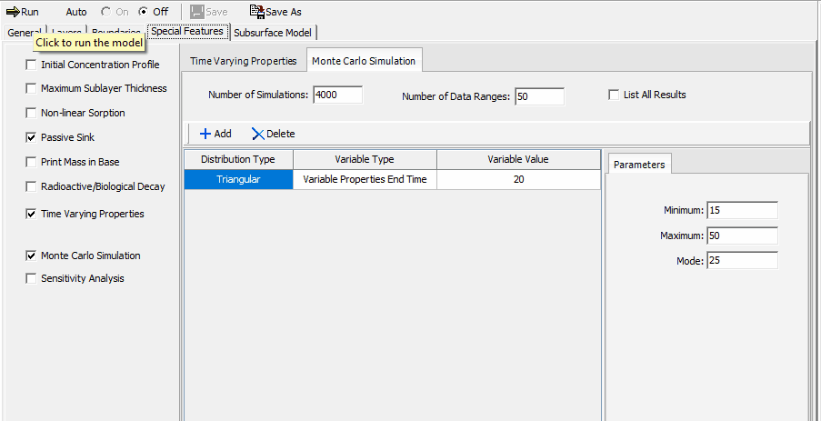
The following can be specified:
Number of Simulations: This is the number of simulation analyses (realizations) to make, during each simulation the probability distributions of each variable are randomly sampled and the concentrations calculated. To obtain sufficiently reliable results at least 500 simulations are recommended, and for some cases between 1000 to 10000 simulations (realizations) may be required. The user should experiment with this parameter to determine the sensitivity of the results to the number of simulations.
Number of Data Ranges: This is the number of data ranges to divide the probability distributions into in the output of the results of the simulation. A maximum of 20 ranges may be specified. This parameter does not affect the accuracy of the results and is for display purposes only.
List All Results: By selecting this option, the user can obtain a list of all the simulation results. Listing all the results will include the results of every simulation pass in the output, the output file that is obtained may be extremely large. This option can be used to list all the results for a limited number of simulations (e.g. 10), to obtain a better idea of how the program is functioning, prior to running it for all the simulations.
Variables
Each variable represents one data item in the input data to be modified in the Monte Carlo simulation and is specified in the variable table. At the top of the table there are buttons to add and delete a variable. For each variable the following is specified:
Distribution Type: A distribution must be entered for each variable, the distribution types can be different for different variables. There are five types of probability distributions that can be entered:
Uniform Distribution: This is used to specify a uniform probability distribution, in which there is the equal probability that a data point has any value between a specified minimum and maximum. The probability distribution curve would be a horizontal straight line. The user will need to specify the Minimum and Maximum data values in the Parameters to the right of the table.
Triangular Distribution: This is used to specify a triangular probability distribution function, where the probability is a maximum for a given value (mode) then linearly drops off on each side of this value. The probability distribution curve would be a triangle. The user will need to specify the Minimum, Mode, and Maximum data values in the Parameters to the right of the table.
General Distribution: This is used to specify a set of data and probability pairs that will be linearly interpolated. The probability distribution curve would be a continuous function, which is approximated by a set of straight line segments. The set of values must cover the entire data range, and the probability values do not have to sum to 1. The data and probability pairs can be entered in the Parameters to the right of the table.
Normal Distribution: This is used to specify a normal distribution for the variable. The distribution is symmetrical in shape similar to a bell, and is sometimes called a Gaussian distribution. To define the distribution the user needs to specify the Mean and Standard Deviation in the Parameters to the right of the table.
Lognormal Distribution: A lognormal distribution can be specified for the variable with this option. This distribution is similar to the normal distribution except that it is based on the logarithm of the random variable (eg. Darcy velocity or layer thickness). The user will need to specify the Mean of the log of the variable and the Standard Deviation of the log of the variable in the Parameters to the right of the table.
Variable Type: This is the type of data for which the user wishes to enter a probability distribution. There are 6 types of data that can be used:
Initial Source Concentration: This is the Initial Source Concentration of the top boundary, and can only be used if the top boundary condition is NOT zero flux.
Darcy Velocity: This is the Darcy Velocity of the model.
Layer Thickness: This allows the user to specify a distribution for the thickness of a layer. The user will be asked to specify the layer for which to vary the thickness.
Diffusion Coefficient: This is the Diffusion Coefficient of a layer, the user will be asked to specify the layer for which to vary the Diffusion Coefficient.
Distribution Coefficient: This is the Distribution Coefficient of a layer, the user will be asked to specify the layer for which to vary the Distribution Coefficient. If the layer selected is fractured the distribution coefficient along the fracture will be varied.
Variable Properties End Time: This is the End Time of a Variable Properties Time Group, the user will be asked to specify the Time Group for which to vary End Time. When varying the end time of a time group the program will shift the end times of subsequent time groups to maintain their relative position, and will try to keep the end times of any previous time groups the same. This variable type will not show up if the Variable Properties feature has not been previously selected.
Variable Value: If the variable type is Layer Thickness, Diffusion Coefficient, or Distribution Coefficient this is the layer to use for the variable. If the variable type is Variable Properties End Time this the end time of the time period to vary.