|
<< Click to Display Table of Contents >> Layers |
  
|
|
<< Click to Display Table of Contents >> Layers |
|
To edit the layer data for a model click on the Layers tab on the left side of the model form.
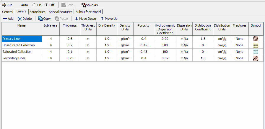
At the top of the tab there are buttons for:
Add: Add a layer below the currently selected layer.
Delete: Delete the currently selected layer.
Copy: Copy the currently selected layer to the clipboard.
Paste: Paste the layer in the clipboard below the currently selected layer.
Move Down: Move the currently selected layer down.
Move Up: Move the currently selected layer up.
The following can be specified for each layer:
Name: This is the name of the layer. It is used only for drawing and output.
Number of Sublayers: The number of sublayers in each layer is primarily used in the output of the calculated concentrations with depth; a concentration will be calculated at each sublayer interface. If the Freundlich Non-Linear Sorption, Langmuir Non-Linear Sorption, or Variable Properties Special Feature is selected, the accuracy of the results will depend on the number of sublayers.
Thickness: This is the thickness of the layer, this is the total thickness of all the sublayers in the layer.. The maximum thickness of each sublayer is 5 units. This maximum can be adjusted using the Maximum Sublayer Thickness option of the Special Features menu. If the maximum sublayer thickness is not changed then the number of sublayers is automatically increased if required to keep their thickness to less than 5.
Dry Density: The dry density of the layer.
Porosity: This is the porosity of the layer, which must be greater than 0 and less than or equal to 1. If the layer is being used to represent a geomembrane the porosity should be set to 1.
Coefficient of Hydrodynamic Dispersion: This is the coefficient of hydrodynamic dispersion for the layer:
D = De + Dmd
where,
De = the diffusion coefficient for the species,
Dmd = the coefficient of mechanical dispersion.
For intact clayey layers, diffusion will usually be the controlling factor and dispersion will often be negligible [Gillham and Cherry, 1982, Rowe, 1987; Rowe et al, 2004]. In sandy layers, dispersion will tend to be the controlling factor. If the Variable Properties option of the Special Features submenu is selected the dispersivity can be specified separately.
Distribution Coefficient: This is the distribution coefficient for the layer. In the basic mode (ie. where Langmuir Non-linear sorption and Freundlich Non-linear sorption have not been selected) the sorption-desorption of a conservative species of contaminant is assumed to be linear such that:
S = Kd c
where,
S = solute sorbed per unit weight of soil,
Kd = distribution (sorption) coefficient,
c = concentration of contaminant.
This is a reasonable approximation for low concentrations of contaminant, however at high concentrations sorption is generally not linear and more complex relationships should be used. If there is no sorption (i.e.,a conservative species) the distribution coefficient is zero. Two types of non-linear sorption can be used if desired, these are Langmuir Non-Linear Sorption and Freundlich Non-Linear Sorption. Both options can be selected in the Special Features submenu.
Fractures: Any or all of the layers may be fractured. These fractures may be 1, 2, or 3 dimensional. Where the first dimension is for one set of vertical fractures, the second is for a second set of (orthogonal) vertical fractures, and the third is for horizontal fractures (ie. for a 3D block, dimension 1 is length, dimension 2 is width, and dimension 3 is depth). If 1, 2, or 3 dimensional fractures are specified for the layer, the fracture data can be entered at the bottom of the tab.
Symbol: This is used to select the symbol that will be used for the layer when drawing the subsurface model. When the symbol is clicked on the symbol can be selected as described in the Select Symbol section.
Fractures
Continuity of concentration and flux is assumed at the boundary between layers. If a fractured layer is in contact with an unfractured layer, it is assumed that all fluid flow is transported along the fractures that intersect the unfractured layers (i.e., it is equivalent to having a very thin sand layer between unfractured and fractured layers). In a fractured model the program can consider advective-dispersive transport along the fractures coupled with diffusion into the matrix on either side of the fracture. However, if the Darcy velocity is zero, or small, then the transport mechanism will be essentially diffusive through the matrix, the fractures will have no effect and should not be considered in modeling the migration of contaminants. Users planning to model migration in fractured media are warned that they should first see Rowe and Booker, 1990, 1991a, 1991b, and Rowe et al, 2004 for a discussion of modeling of fractured systems.
The following information about the fractures in each dimension can be specified:
Fracture Spacing: The spacing of fractures is the distance between fractures in each dimension.
Fracture Opening Size: The fracture opening size is the width of the gap between the fracture walls.
Number to sum: This is the number of terms to sum in the evaluation of the advective-dispersive equation for contaminant migration [Rowe and Booker, 1990, 1991a, 1991b]. For blocks where the fracture spacing is of the same order in all directions, 8 to 10 terms is usually adequate. As the aspect ratio (horizontal spacing/vertical spacing or vertical spacing/vertical spacing) increases more terms are required in the summation. When the aspect ratio is large, the problem can usually be reduced to a lower order (eg. from 3D to 2D or 2D to 1D). For example, if the spacing between fractures in one vertical direction is 50 units, and in the other vertical and horizontal directions is 2 units. The widely spaced fractures can be ignored and the problem reduced to a 2D problem [Rowe and Booker, 1990].
Dispersion coefficient: This is the dispersion coefficient along the fracture.
Distribution coefficient: This is the distribution coefficient along the fracture as defined by Freeze and Cherry (1979). This is often assumed to be zero.
Select Symbol
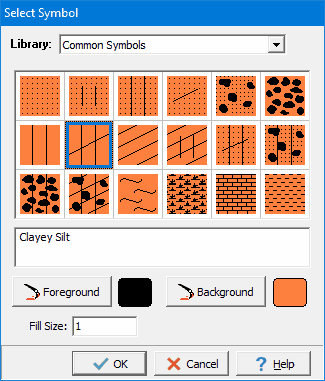
The following information can be specified using this form:
Library: This combo box is used to select the symbol library to use to draw the layer. When the arrow at the right is pressed a list will display the available symbol libraries. After a library has been selected, the symbols displayed in the tab will be updated.
Symbol: The symbol from the library can be selected by clicking on one of the 18 symbols displayed for the current library. The selected symbol is highlighted with a blue border.
Foreground Color: This is the color to use for the shaded parts of the symbol. The foreground color can be changed by pressing the Foreground Color button. When this button is pressed a Color form is displayed. Using this form, a basic color can be selected or a custom color can be specified.
Background Color: This is the color to use for the unshaded parts of the symbol. The background color can be changed by pressing the Background Color button. When this button is pressed a Color form is displayed. Using this form, a basic color can be selected or a custom color can be specified.
Fill Size: The fill size is used to expand or condense the symbol The size of the symbol is multiplied by the fill size and then the symbol is drawn. For example, a fill size of 2 will result in the symbol being doubled in size. The fill size must be greater than 0.